Statistics is an intriguing subject that helps interpret the world around us. Researchers and governments use it to discover new phenomena and to establish claims. The 21st-century business environment strategy is hugely guided by data. This article is a broad overview of descriptive Statistics concepts, we will dive deeper into the topics in subsequent articles.

What Is Statistic

Statistics is the branch of mathematics that deals with the collection, analysis, interpretation, and presentation of data. It is divided into two categories: inferential and descriptive Statistics.

Data professionals use inferential Statistics to make inferences, and predictions and draw conclusions on unknown data, while descriptive Statistics allow them to summarize data.

What is a descriptive Statistic?

Descriptive Statistics is used to describe and summarise datasets. The central tendency and measures of dispersion are at the centre of data summarization.

Three important metrics are involved when it comes to the central tendency. They are the mean, median and mode. The standard deviation, variance and range depict the distribution of a data set. In this brief overview, we will discuss the list below. So let us get started:

• The measures of central tendency
• Measures of variability or dispersion
• Range
• Variance
• Standard deviation
• Skewness
• Ketosis
• Frequency distribution

The mean mainly called the average is the central point of a dataset where most of the data lies. The median is the value that separates the upper half values from the lower half values when the data set is arranged in numerical order. The mode is the frequently occurring value in a dataset.

The standard deviation shows the average dispersion of data points in the distribution, and the variance is the squared average dispersion about the mean. When you take the maximum value in a data set and subtract from it the minimum value, you come up with the range.

The frequency distribution arranges data in a table format or chart for easy and quick use and capturing occurrences. Data in a frequency distribution can be grouped and shown in percentages.

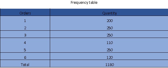
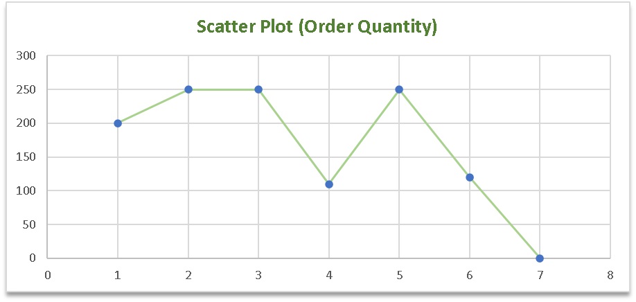
So, given the frequency table below, the average, median and mode order quantity values will be 196.67, 255 and 250 in this order. The measures of dispersion will also produce the following values for the standard deviation and variance in that order: 66.23, 43.87 and the range value of 140.

Here is the frequency table on ordered items and the quantity ordered for each item.

Frequency table



It is important to understand some foundational concepts about Statistics. The object of interest or study is called a population. But very rarely do data professionals use the population in their research. They take a sample of the population and use the sample parameters to make predictions or draw conclusions about the population parameters. Most datasets are a normal distribution and have a bell shape.

The normal distribution provides a clear picture of a data set, where the mean lies in the centre and peak of the chart. 68 per cent of the data lies within (+-) one standard deviation, 95 per cent of the data lies within (+-) two standard deviations and 99% of the data lies within (+-) standard deviation. It is important to understand some foundational concepts about Statistics. The object of interest or study is called a population.

But very rarely do data professionals use the population in their research. They take a sample of the population and use the sample parameters to make predictions or draw conclusions about the population parameters. Most data sets are a normal distribution and have a bell shape.

The normal distribution provides a clear picture of a data set, where the mean lies in the centre and peak of the chart. 68 per cent of the data lies within (+-) one standard deviation, 95 per cent of the data lies within (+-) two standard deviations and 99% of the data lies within (+-) standard deviation.

Skewness measures asymmetrical or the lack of it in a distribution. Using the right and left skew to explain, it allows data professionals to understand the shape of a distribution. With its tails also, Ketosis is good at uncovering shapes as it measures the peak and heaviness of a distribution. These topics will be covered in detail in different articles.

Graphical Representation

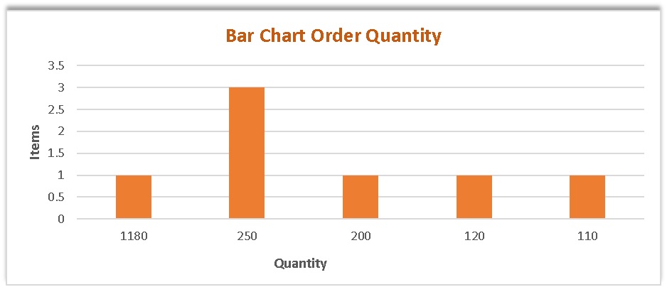
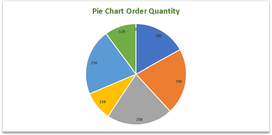
Charts and diagrams are used to describe and summarise the data for quick understanding. The bar chart and the pie chart depict proportions in categorical data. Here is an example of a bar chart.



Below is a pie chart



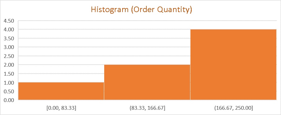
Histogram shows the data distribution.



The scatter plot is used to show relationship between variables.



The box plot excels particularly at revealing outliers and further illustrates the range, interquartile range and median range. The boxplot is fully covered in another article.

Conclusion

This article provided a broad overview of descriptive Statistics, introducing key concepts that help summarize and describe datasets. Descriptive Statistics plays a crucial role in data analysis by allowing researchers and professionals to understand the characteristics of their data before conducting further statistical modelling or inference.

We covered the two main components of descriptive Statistics - measures of central tendency (mean, median, mode) and measures of variability (range, variance, standard deviation). These metrics provide insights into the central values and spread of a distribution. We also touched on distribution shapes like skewness and kurtosis that reveal asymmetry and peakness.

Additionally, we highlighted the importance of graphical representations such as bar charts, pie charts, histograms, scatter plots, and box plots in visualizing data for quicker interpretation. Frequency distributions, both grouped and ungrouped, organize data for easier understanding.

While this served as a brief introduction, each of these descriptive Statistics concepts warrants a deeper dive. In subsequent detailed articles, we will explore the calculations, properties, and applications of the mean, median, mode, range, variance, standard deviation, skewness, kurtosis, frequency distributions, and data visualization methods.

Having a solid grasp of descriptive Statistics is foundational for any data professional. It allows you to effectively summarize, interpret, and communicate insights from complex datasets. This overview has set the stage for a comprehensive understanding of this crucial field through the upcoming in-depth articles.